| Brief Description | |
|---|---|
|
Files:
\examples\Processing\HDR_ImageComposition\HighDynamicRange\HDR_linearW_Bayer_3_Base.vad |
 |
|
Default Platform: mE5-MA-VCL |
|
|
Short Description Weighted Linear HDR Algorithm and LDR Algorithm according to Reinhard et al. and Fattal et al.. |
|
This High Dynamic Range (HDR) and Low Dynamic Range (LDR) VisualApplets (VA) design is similar to the one described in 'High Dynamic Range and Low Dynamic Range Example Using Camera Response Function'. The difference is the HDR algorithm. This will be described in the following subsection. There exist several variations of this example: They are designed for a marathon VCL board in base and full configuration for a RGB, a Bayer pattern or a grayscale camera.
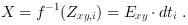
The exposure  can be written
as inverse function of Equation 32
can be written
as inverse function of Equation 32
If you can suppose the exposure to be a linear function you can construct the HDR color components with:
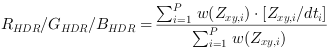
instead of with Equation 34. Here
 is analog to Equation 35 a weighting function with which under and over exposed pixel values are less emphasized. The LDR components in this
example are calculated analog to the LDR algorithms in and .
is analog to Equation 35 a weighting function with which under and over exposed pixel values are less emphasized. The LDR components in this
example are calculated analog to the LDR algorithms in and .
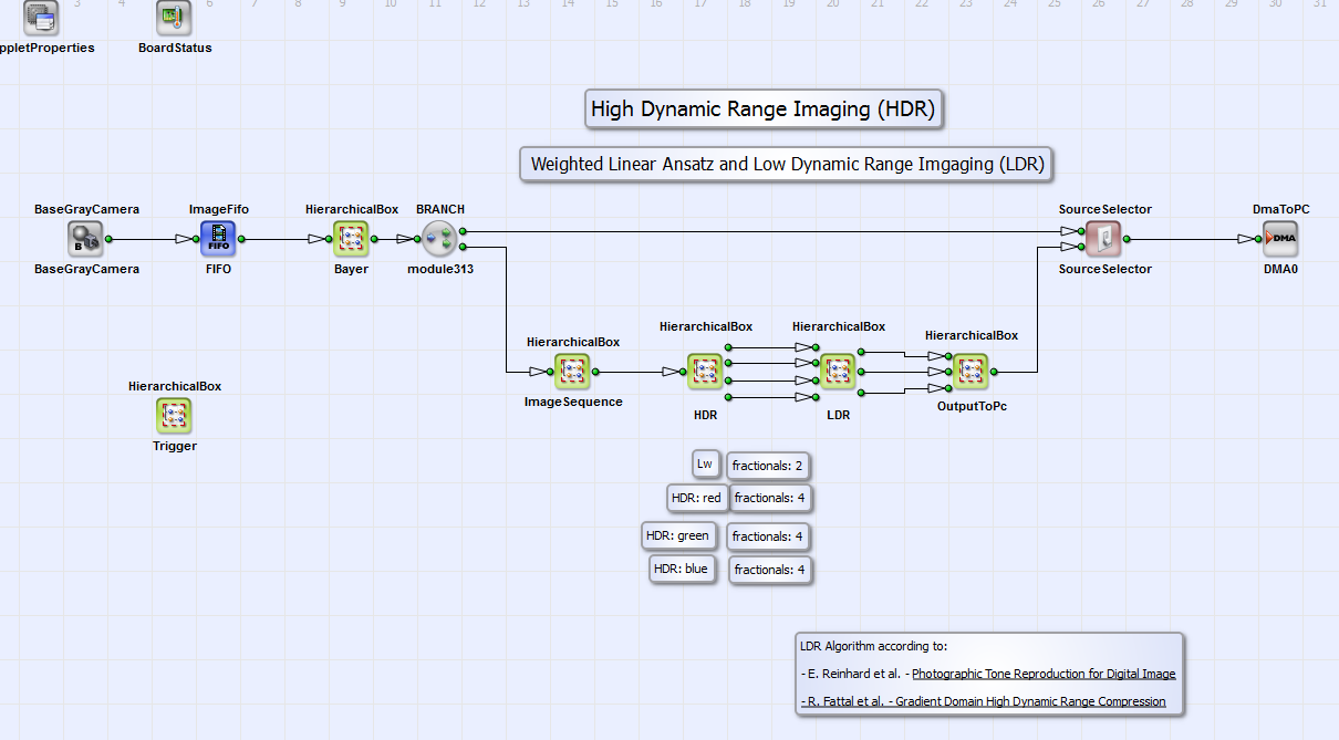
The example is suitable for filming scenes with very wide luminosity scale with very dark and very bright objects. An image is transferred to PC in which every object of the scene is displayed properly. The basic structure of the design is shown in Fig. 352 (here for a Bayer pattern camera in base configuration). The red, green and blue values for every image pixel are calculated in the HierarchicalBox Bayer with a Bayer5x5Linear operator. In the box ImageSequence a sequence of three images is buffered. The three images should have three different exposure times for HDR-LDR processing. The exposure times should be chosen that way that every image pixel is at least in one image of the exposure sequence neither under nor over exposed. You can set these times with the operators SignalWidth width1 to width3 in the HierarchicalBox Trigger (see Fig. 346). Please note that the time scale is system clock ticks of 8 ns. The operator Generate-Period has to be set at least to a value greater than the longest time of the operators SignalWidth width1 to width3. Please read in addition the minimum period length for operator Generate-Period in your camera manual. The three images are combined using the weighted linear HDR algorithm described in Equation 43. It is implemented in the HierarchicalBox HDR (Fig. 352). The LDR algorithm according to Reinhard et al. [Rei02] and Fattal et al.[Fat02] is implemented in LDR. The colors of the resulting RGB image are merged in the HierarchicalBox OutputToPC. In the design "HDR_linearW_Gray_3_Base.vad" this box does not exist. The operator SourceSelector gives the opportunity to select the DMA transport of either the processed HDR-LDR image or the (Bayer demosaiced) camera image. Since the design structure and calculations are analog to the ones of the example in section we will just concentrate on the explanation of the content of HDR in the following. But please note that in some details like fractional bits the designs might also differ. You find the corresponding hints in the comment boxes in the examples.

In Fig. 353 you can see the content of the HierarchicalBox HDR. For the three images of the buffered
image sequence the summands of the nominator
 and denominator
  of Equation 43 are calculated
for images one to three (HierarchicalBox Image1 to Image3) for the colors red, green and blue separately. For grayscale images in the design
"HDR_linearW_Gray_3_Base.vad" the calculation is done for the grayscale component only .
of Equation 43 are calculated
for images one to three (HierarchicalBox Image1 to Image3) for the colors red, green and blue separately. For grayscale images in the design
"HDR_linearW_Gray_3_Base.vad" the calculation is done for the grayscale component only .

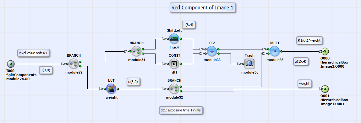
The calculation of these summands is shown in Fig. 354 for color red in Image1 as example. The
calculation for the colors green and blue and images 2 and 3 are analog. The pixel value in Fig. 354 is divided by the exposure
time which can be set by the value of the parameter Const_dt1 (or analog Const_dt2 and Const_dt3).
The time base can be seconds, milli- or microseconds and can be set by the parameter
TimeBase in the boxes 红色, 绿色 and 蓝色 in the box HDR
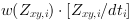
(see Fig. 353 and Fig. 355). The result of
 is multiplied with a weighting function implemented
as lookup table LUT_weight. The table "WeightsLinear.txt" can be created using the Matlab program modules "WeightLinear.m", "sample.m"
(or "sample_gray.m" for grayscale images) and "HDR_CRC_m"
(or "HDR_CRC_Gray.m" for grayscale images)
(under \examples\Processing\Advanced\HighDynamicRange\). Please read also the short manual in "HDR_CRC.m" (or "HDR_CRC_Gray.m"
for grayscale images) for further instructions.
The outputs of the component shown in Fig. 354 are then the summands of Equation 43:
is multiplied with a weighting function implemented
as lookup table LUT_weight. The table "WeightsLinear.txt" can be created using the Matlab program modules "WeightLinear.m", "sample.m"
(or "sample_gray.m" for grayscale images) and "HDR_CRC_m"
(or "HDR_CRC_Gray.m" for grayscale images)
(under \examples\Processing\Advanced\HighDynamicRange\). Please read also the short manual in "HDR_CRC.m" (or "HDR_CRC_Gray.m"
for grayscale images) for further instructions.
The outputs of the component shown in Fig. 354 are then the summands of Equation 43:
 and
and  .
.

These summands are summed up and divided according to Equation 43 in the HierarchicalBoxes Red, Green and Blue. See for example box Red in Fig. 355.
The calculation of the luminance
 in the module Luminance, of the scaled luminance
 ,
of the LDR luminance
,
of the LDR luminance
 and the final calculation
of the LDR color components
and the final calculation
of the LDR color components
 ,
,
 and
and
 或
或
 is analog to the implementation in section 'High Dynamic Range and Low Dynamic Range Example Using Camera Response Function'. Please refer for further reading the corresponding
parts in section or the comment boxes in the VA design.
is analog to the implementation in section 'High Dynamic Range and Low Dynamic Range Example Using Camera Response Function'. Please refer for further reading the corresponding
parts in section or the comment boxes in the VA design.
